
Integrating Spatial Transcriptomics with Single-cell RNA-seq
How to integrate spatial transcriptomics with scRNA-seq: when spatial context helps, the key integration methods, and worked tissue examples.

Single-cell and spatial transcriptomics series, Part 2 of 3. Part 1 covers when scRNA-seq alone is enough. This part covers integrating spatial data, and Part 3 looks at where the two technologies converge.
Part 1 covered how much you can learn from scRNA-seq on its own, and where it runs into a wall: dissociating a tissue discards where each cell sat and who it neighboured. Spatial transcriptomics puts that arrangement back, mapping gene expression onto tissue architecture. This part covers when spatial context is worth adding to a single-cell study, the main methods for integrating the two data types (Seurat label transfer, SpaGE, Tangram, pciSeq, BayesSpace, and deconvolution tools such as cell2location), and worked examples where even a small spatial experiment sharpens a large single-cell dataset.
Why spatial context matters for single-cell data
scRNA-seq profiles what each cell expresses but loses where the cell was. Tissues are not random collections of cells; they have structure, such as cortical layers in the brain, niches in bone marrow, tumour-immune neighbourhoods, and developmental gradients in an embryo. A cell's identity and function are often tied to its position and neighbours, so dropping location can hide organisation that matters.
One way to picture it: scRNA-seq gives you the cast and their lines, the cell types and what each expresses. Spatial transcriptomics adds the stage directions, where each cell stands and who it is next to. With both, you can read the whole scene. Concretely, adding spatial data lets you:
- See tissue architecture. How cell types are arranged into anatomical structures, for example layered neurons in cortex, zonation in liver lobules, or immune cells massing at an infection site.
- Find cell interactions. Which cell types co-localise or form neighbourhoods, which points to cell-cell communication, for example T cells nestled against cancer cells at a tumour margin.
- Map developmental gradients. Positional cues such as morphogen gradients across an embryo that correspond to developmental changes in gene expression.
- Read cell states in context. An "activated" immune cell inside a tumour and one in a lymph node carry different implications, and location is what tells them apart.
Spatial context turns a list of cell types into a map of cellular geography. It lets you ask not only what cell types are present and what they express, but where they are and how location shapes their behaviour.
A primer on spatial transcriptomics methods
Spatial transcriptomics (ST) covers techniques that measure gene expression while keeping track of where in the tissue each measurement came from. They split into two broad classes, with different trade-offs between resolution and gene coverage.
| Approach | Examples | Resolution | Gene coverage |
|---|---|---|---|
| Imaging-based (probes imaged in situ) | seqFISH, MERFISH, CosMx, Xenium | Single-cell, down to subcellular | Targeted panel, tens to ~1,000 genes |
| Sequencing-based (spatially barcoded capture) | 10x Visium and Visium HD, Slide-seq, Stereo-seq | Spot-level on classic Visium (~55 µm, ~1-10 cells) up to single-cell scale on Visium HD (2 µm) and Stereo-seq | Whole transcriptome, unbiased |
The trade-off has narrowed since these methods first appeared. Until recently, no spatial platform gave you both the whole transcriptome and single-cell resolution across a tissue, which is what made integration with scRNA-seq essential. That gap is closing: since 2024, Visium HD resolves whole-transcriptome expression at 2 µm across the capture area, approaching single-cell scale, and imaging platforms such as Xenium and CosMx are already single-cell (Oliveira et al., 2025). Integration is shifting accordingly, from deconvolving multi-cell spots toward annotating and segmenting cells that are already resolved. Deconvolution still matters, though, for classic Visium and for coarser binning of high-resolution data, and scRNA-seq remains the reference that gives spatial data its cell identities and full gene coverage.
When does spatial data enhance scRNA-seq?
Not every single-cell study needs spatial data. A few situations gain a lot from it:
- Complex tissue architecture. In a structured tissue (brain, gut, kidney, tumour with microenvironment), spatial data maps discovered cell types back to anatomy. A brain scRNA-seq might find several neuron subtypes; spatial mapping shows they form distinct layers, confirming known organisation or revealing new structure.
- Cell-cell interactions in disease. In cancer or inflammation, who sits next to whom is often the biology. A tumour scRNA-seq can identify T cells and cancer cells, but spatial data shows whether the T cells cluster at the invasive margin or around vessels. A glioblastoma study integrating the two mapped malignant and immune cells in the tumour and found specific macrophage and T cell populations co-localising and signalling via ligand-receptor pairs (Liu et al., 2023).
- Developmental gradients and niches. During development, position is the point. Integrating even a targeted spatial panel with an scRNA-seq atlas can reveal head-tail, inside-outside, or dorsal-ventral gradients. Profiling an 8-12 somite mouse embryo with seqFISH for 387 genes and integrating it with scRNA-seq atlases exposed a dorsal-ventral patterning of gut-tube progenitors that dissociated data alone did not show (Lohoff et al., 2022).
If the question is about how cells are arranged, who they neighbour, or how location shapes behaviour, spatial data earns its place. The encouraging part is that you rarely need a large spatial experiment; a single Visium slide or one targeted imaging panel can complement a big scRNA-seq dataset, as long as the integration is done well.
Strategies to integrate single-cell and spatial transcriptomics data
Methods for combining the two data types fall into a few categories: label transfer and mapping, imputation of unmeasured genes, deconvolution of multi-cell spots, and spatial domain detection. The methods below cover most of what single-cell researchers reach for first.
| Method | Category | What it does | Reach for it when |
|---|---|---|---|
| Seurat label transfer (anchors) | Label transfer / mapping | Transfers cell-type labels from an annotated scRNA-seq reference onto spatial cells or spots via shared anchors | You have a well-annotated reference and want to label spatial data |
| SpaGE | Imputation | Predicts unmeasured genes in spatial data from an scRNA-seq reference | Your spatial panel is small and you want broader gene coverage in situ |
| Tangram | Mapping | Learns a deep-learning mapping that places scRNA-seq cells onto spatial coordinates | You want to project single cells, annotations, or genes onto tissue |
| pciSeq | Probabilistic cell typing | Assigns cell types to in situ sequencing reads using an scRNA-seq reference | You have imaging-based in situ data and need per-cell type calls |
| BayesSpace | Spatial clustering / resolution | Uses spatial neighbourhood information to sharpen spot clusters and push toward sub-spot resolution | You want to refine Visium spot clusters spatially |
| RCTD (spacexr) | Deconvolution | Estimates cell-type proportions per spot from an scRNA-seq reference while modelling platform effects | You want robust spot deconvolution, including for Visium HD bins |
| SpatialDWLS | Deconvolution | Weighted least-squares estimation of cell-type composition at each location | You want fast, accurate spot deconvolution |
These are a selection, not the whole field. Others include cell2location, STdeconvolve, Stereoscope, novoSpaRc, and Harmony for multi-modal integration. Independent benchmarking helps narrow the choice: across 16 integration methods on 45 paired datasets, Tangram, gimVI, and SpaGE were strongest for predicting the spatial distribution of unmeasured transcripts, while cell2location, SpatialDWLS, and RCTD led on cell-type deconvolution of spots (Li et al., 2022). A sensible default is to pick by task: label transfer or mapping (Seurat, Tangram) when you need per-cell identities, deconvolution (cell2location, RCTD, SpatialDWLS) when spots still mix several cells, and imputation (SpaGE, Tangram) for genes the spatial panel did not measure.
A worked example: tumour biopsy plus one Visium slide
Suppose you have 50,000 cells from a tumour biopsy and suspect the spatial arrangement of tumour, immune, and stromal cells matters, but budget only stretches to a single 10x Visium slide. Each Visium spot is a whole-transcriptome readout averaged over several cells. A practical route through it:
- Analyse the scRNA-seq first. Cluster and annotate the major cell types (tumour cells, T cells, macrophages, and so on). ScarfWeb handles the clustering and annotation without code.
- Transfer onto spots. Use a deconvolution or label-transfer method (cell2location, RCTD, or Seurat) to estimate what each spot contains, for example spot 123 is 50% tumour, 30% T cell, 20% macrophage. On a single-cell-resolution platform such as Visium HD or Xenium you would segment and annotate cells directly rather than deconvolving spots.
- Read the tissue map. A common pattern emerges: tumour-core spots are mostly tumour cells with few T cells, while edge spots are T-cell rich, consistent with immune infiltration at the margins.
- Refine where it counts. BayesSpace can subdivide spots in high-T-cell regions, and you can inspect checkpoint-ligand expression in spatial context to follow up on interactions.
A few checks that save you later. Make sure the datasets truly correspond, ideally the same tissue or condition, and correct any batch differences before or during integration (Harmony or Seurat's CCA help). Validate where you can: Lohoff and colleagues confirmed imputed expression against in situ staining. Ground truth is not always available, but sanity checks (do known markers localise correctly, do integrated clusters match histology) raise confidence.
Real-world examples
A few cases where integrating spatial data with single-cell transcriptomics changed what the study could see:
- Brain cortex, layered architecture. scRNA-seq alone does not assign cells to cortical layers. In a frontal cortex study, a large Drop-seq dataset (~71k cells) was integrated with a smaller STARmap spatial dataset (~2.5k cells) using LIGER, which let each single-cell cluster be placed in a layer (Welch et al., 2019). Interneuron subtypes mapped to layer 1 at the surface, others to deep layers. The integration also sharpened the sparser spatial dataset, with breadth from scRNA-seq and an anatomical map from spatial reconstructing the tissue in silico.
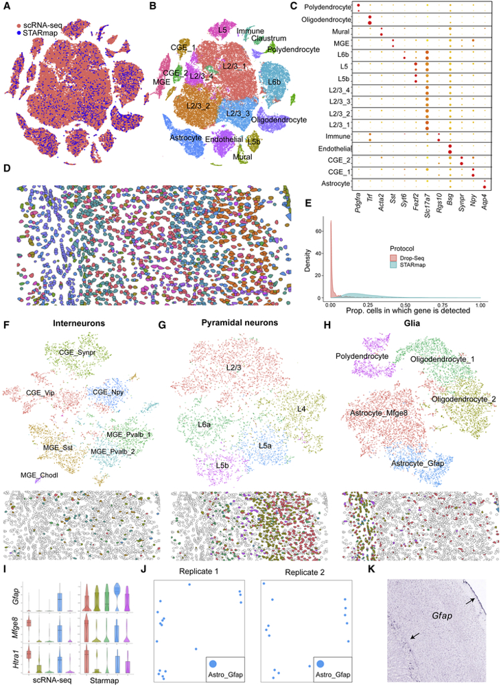
Figure 1: Integrating scRNA-seq with spatial data reveals cortical organisation. A large dissociated single-cell dataset (71k cells) was integrated with a smaller STARmap spatial dataset (2.5k cells). After joint clustering, the STARmap cells were plotted on their spatial coordinates and coloured by cluster identity, mapping the scRNA-seq clusters onto the tissue and recapitulating known cortex anatomy (Welch et al., 2019).
-
Tumour-immune microenvironment. Mapping the tumour microenvironment is now a flagship use of single-cell-resolution spatial data. A 2025 study profiled human colorectal cancer with Visium HD at single-cell scale, alongside matched scRNA-seq and Xenium, and resolved transcriptionally distinct macrophage subpopulations occupying different niches with pro- and anti-tumour roles, defined through their interactions with tumour and T cells (Oliveira et al., 2025). In situ analysis localised a clonally expanded T cell population next to macrophages with anti-tumour features. Knowing which cells actually touch each other is what turns a cell-type list into a candidate target. Interaction analysis of this kind is now typically run with frameworks like LIANA, which aggregate several ligand-receptor methods into one consensus (Dimitrov et al., 2022); the long-standing CellPhoneDB is now at v5.
-
Developmental gradients in an embryo. The Lohoff study is worth detailing because it shows how little spatial data you can get away with. The researchers had a comprehensive single-cell atlas of mouse embryogenesis and ran seqFISH on embryo sections for just 387 marker genes. By matching each spatial cell to its nearest atlas cell, they imputed the rest of the transcriptome and built a near-complete spatial expression map (Lohoff et al., 2022). That map revealed an early dorsal-ventral split of gut-tube cell fates the atlas alone had missed. The general lesson: a small, well-chosen spatial experiment can amplify a large single-cell dataset, and SpaGE and Tangram are well suited to this kind of imputation and alignment.
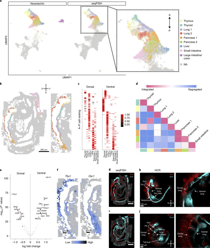
Figure 2: Spatial mapping of a mouse embryo from a small seqFISH panel integrated with an scRNA-seq atlas. Each dot is a cell, coloured by predicted cell type. Integration let the authors assign a type to each cell and infer genes not measured by seqFISH, exposing a dorsal-ventral separation of future trachea (ventral) and oesophagus (dorsal) progenitors along the gut tube. The pattern was confirmed by in situ hybridisation for markers such as Tbx1 and Shh and was not evident from dissociated data alone (Lohoff et al., 2022).
Adding spatial context in ScarfWeb
Most of these integrations can be done without building a pipeline from scratch in R or Python. ScarfWeb, Nygen's single-cell platform, runs the scRNA-seq side (quality control, clustering, differential expression) through a graphical interface, and it lets you import spatial coordinates for your cells or spots and visualise expression or clusters on the tissue layout. In practice that means once you have identified clusters in the single-cell data, you can overlay them on the original tissue positions and read off spatial patterns without custom code. The knowledge-base article on importing spatial and clonotype data walks through uploading x,y coordinates and pairing them with the expression data.
Where this leaves us, and what Part 3 covers
Integrating spatial transcriptomics with single-cell RNA-seq lets you see how cells work together in tissue, not just what they are. Even limited spatial information, paired with solid single-cell data, can resolve tissue architecture, pinpoint cell interactions, and expose patterns like developmental axes that dissociated analysis misses. The craft is matching the integration method to the question, from simple label transfer for annotating regions to probabilistic mapping for predicting unmeasured genes. Seurat, SpaGE, Tangram, pciSeq, BayesSpace, and deconvolution tools such as cell2location each cover a different part of that problem.
As both technologies advance, the boundary between "scRNA-seq" and "spatial" is thinning. Part 3 treats them as complementary tools rather than competing options, and looks at the emerging platforms, machine-learning integration methods, and spatial multi-omics that are pushing the two together.
Related articles
The biology in your ligand-receptor analysis, and how to read it
Ligand-receptor analysis is easy to run and easy to over-read. How to get cell-cell communication biology from the ranked table, with LIANA and ScarfWeb.
Read more →
Multi-Omics Data for Target ID in Drug Discovery
How human genetics, single-cell transcriptomics, chromatin accessibility and proteomics combine into causal, cell-resolved target evidence, where integration usually fails, and how to grade the result before a programme is committed.
Read more →
Spatial Transcriptomics and scRNA-seq: A Complementary Pair
The current state of spatial transcriptomics and scRNA-seq: single-cell-resolution platforms, foundation models for integration, spatial multi-omics, and 3D tissue atlases.
Read more →