
When is Single-cell RNA-seq Enough, and When Do You Need Spatial Data?
When is scRNA-seq enough on its own? A guide to its use cases, the workflow from clustering to cell type annotation, and when to add spatial data.

Single-cell and spatial transcriptomics series, Part 1 of 3. This part covers when scRNA-seq alone answers the question. Part 2 covers integrating spatial data, and Part 3 looks at where the two technologies converge.
Single-cell RNA sequencing (scRNA-seq) profiles gene expression one cell at a time, which exposes the cellular heterogeneity that bulk RNA-seq averages away. That resolution is why it has become the default first experiment for studying development, disease, and treatment response. It also raises a practical question that decides how much time and budget an experiment needs: when is scRNA-seq on its own enough, and when do you actually need to add spatial context?
This first part works through the scenarios where scRNA-seq alone is sufficient, walks through the core analysis workflow from clustering to cell type annotation to trajectory inference, and flags where the loss of spatial information starts to cost you. Where it helps, we note how ScarfWeb, Nygen's browser-based single-cell platform, runs these steps without code.
What scRNA-seq captures that bulk RNA-seq misses
Bulk RNA-seq reports one averaged transcriptome for a whole sample. A rare population, or a subtle shift confined to one cell type, disappears into that average. scRNA-seq measures the transcriptome of individual cells, so it resolves what the average hides. In practice that buys you a few distinct things:
- Cell subtypes and rare populations. Per-cell expression separates closely related states that bulk cannot, for example distinguishing T and B cell subsets in immune profiling, or picking out a handful of stem cells or circulating tumour cells in a large sample.
- A census of what is present. Droplet platforms such as 10x Genomics Chromium routinely profile tens of thousands of cells per run, and studies now scale to hundreds of thousands or millions. That breadth gives a fairly complete inventory of the cell types in a tissue.
- Genome-wide expression per cell. Most scRNA-seq protocols measure thousands of genes per cell, so you can discover new markers and gene programmes without deciding in advance what to look for. Many spatial methods, by contrast, either target a fixed gene panel or read out several cells at once.
- Dynamic processes. Because you capture cells across a range of states, you can order them along an inferred axis, or pseudotime, to reconstruct differentiation or a response to stimulus. scRNA-seq often shows not just which cell types are present, but how cells move from one state to another.
These strengths make scRNA-seq a natural starting point. In immunology, where cells dissociate easily and identity is defined transcriptionally rather than by location, scRNA-seq has mapped T cell states and B cell clones from blood and lymphoid tissue without needing tissue coordinates. In cancer, it resolves tumour subclones and rare immune populations in the microenvironment, which matters for understanding heterogeneity and therapy resistance.
The trade-off is spatial. Dissociating a tissue tells you which genes a cell expresses, but not where the cell sat or which cells it neighboured. The useful question is not whether that loss matters in general, but in which specific cases it does not affect the biology you are trying to read.
When scRNA-seq alone is enough
If the goal is to identify cell states and types and the expression changes between them, rather than their physical arrangement, scRNA-seq usually answers it on its own. The four scenarios below cover most of these cases. The third column is deliberately included: it names what you give up, which is also the signal for when to reach for spatial data in Part 2.
| Use case | Why scRNA-seq alone works | What you give up without spatial |
|---|---|---|
| Immune profiling and atlas building | Immune cells dissociate cleanly, and their identity is defined by transcriptome rather than location. Clustering plus marker-based differential expression resolves subsets (for example TH1 vs TH2 signatures). | Where an "activated" cell actually sits. An activated T cell in a tumour and one in a lymph node mean different things. |
| Rare cell type discovery | Single-cell resolution isolates the expression profile of a population that may be 0.1% of the sample, which averaging methods miss entirely. | The tissue niche the rare cells occupy. This can be followed up later with targeted imaging. |
| Developmental and differentiation trajectories | Pseudotime orders cells along a transcriptomic continuum, recovering lineage relationships and the transcription factors that switch at branch points. | Whether the inferred trajectory maps onto a physical gradient in the tissue. |
| Cell-type-specific differential expression | Comparing matched cell types across conditions (disease vs healthy, treated vs control) pinpoints molecular changes, such as an inflammatory programme in microglia in a diseased brain. | How those states redistribute spatially, for example whether the affected cells cluster in particular regions. |
For multi-sample comparisons, batch effect correction is the step that decides whether a difference is real or technical. Most frameworks (Seurat, Scanpy) provide integration methods, and getting normalisation and correction right is what lets you trust that a "treatment effect" is not a sequencing-run artefact. We cover this in more depth in batch effect correction in scRNA-seq data.
Plenty of landmark work rests on scRNA-seq alone: defining new neuron types, resolving haematopoietic differentiation hierarchies, and pinpointing a drug's cellular target by tracking which cell type's expression shifts on treatment. If your question is about what cell types and states exist, what they express, and how that changes across conditions or pseudotime, the combination of clustering, differential expression, and trajectory inference typically gets you there.
The core scRNA-seq analysis workflow
A fairly standard workflow has settled into place. Running each step deliberately, rather than accepting defaults, is usually what separates a defensible analysis from a misleading one. The table lays out the steps, the tools most people reach for, and the mistake each step tends to invite. For an independent, benchmark-backed reference on these choices, the single-cell best-practices guide from Heumos and colleagues is a good anchor (Heumos et al., 2023, Nature Reviews Genetics).
| Step | What it does | Common tools | Watch-out |
|---|---|---|---|
| QC and normalisation | Filters low-quality cells and doublets, corrects for library-size differences | Scanpy, Seurat; Scrublet or DoubletFinder for doublets | Over-aggressive filtering can discard the rare populations you set out to find |
| Dimensionality reduction and clustering | PCA then UMAP for structure; graph-based community detection groups similar cells | PCA, UMAP; Leiden clustering (Scanpy), graph clustering (Seurat) | Cluster resolution is a choice, not a ground truth. Over-cluster, then merge what is biologically identical |
| Cell type annotation | Assigns biological identity to clusters from marker genes, reference mapping, or AI annotation | Marker-gene differential expression, reference mapping, automated and AI annotators | Reference bias; confirm assignments against independent markers |
| Differential expression and pathways | Finds cluster markers and condition differences within a cell type | Wilcoxon and other DE tests; GSEA, over-representation analysis | For condition contrasts, aggregate to pseudobulk per sample rather than testing per cell, or false positives inflate |
| Trajectory and pseudotime | Orders cells along inferred developmental or response continua | Monocle 3, Slingshot, RNA velocity (scVelo) | Trajectory methods assume continuity; validate branch points against known biology |
| Integration and batch correction | Aligns multiple samples so cells group by biology, not by donor or batch | Harmony, Seurat, BBKNN, scVI | Over-correction can erase the biological differences you care about |
Cluster annotation is where domain knowledge does the heavy lifting, and where a lot of downstream interpretation is won or lost. Marker-gene inspection (for example CD3E and CD4 pointing to helper T cells), reference mapping, and AI-based annotators are all in common use, and they are increasingly combined rather than treated as alternatives. Our practical guide to scRNA-seq cluster annotation works through marker curation and automated approaches in detail. Once identities are set, differential expression and pathway analysis turn the census into mechanism. Finding that fibrotic-lung fibroblasts upregulate TGF-β signalling relative to healthy fibroblasts, for instance, is a mechanistic lead that comes entirely from the transcriptome.
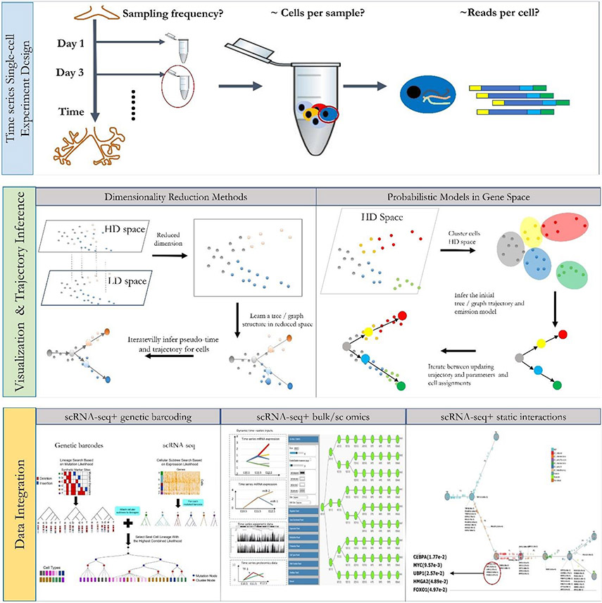
Figure: Overview of a typical single-cell RNA-seq analysis pipeline. After isolating single cells and sequencing their RNA, analysis proceeds through visualisation and clustering to identify cell groups, then trajectory inference to order cells along developmental paths, and integration of multi-sample data where needed (Ding et al., 2022).
Running the analysis without writing code
This workflow assumes comfort in R or Python, which many wet-lab scientists reasonably do not have. Browser-based platforms close that gap by exposing the same steps through a graphical interface, with the established algorithms running underneath. ScarfWeb, Nygen's single-cell platform, handles the pipeline above end to end: upload raw data, then move through normalisation, clustering, marker identification, trajectory inference, and batch correction without scripting. Multi-sample datasets are detected and integrated automatically, so cells from different samples land in one shared embedding ready for comparison.
Annotation and interpretation are assisted too. Clusters can be labelled with AI-assisted cell type annotation, and genes or pathways of interest are surfaced against reference databases, which cuts the chance of missing a signal. The platform keeps a version-tracked record and runs in the cloud, so an analysis can be shared as an interactive view with collaborators or a bioinformatics core rather than passed around as large files. If you want the background on why no-code tooling matters for wet-lab researchers, see overcoming bioinformatics skill gaps in single-cell research.
Where scRNA-seq ends and spatial begins
scRNA-seq answers a specific set of questions well: what cell types and states are present, what they express, how that expression differs across conditions, and how states relate along a trajectory. What it cannot tell you is where those cells were or which cells they touched. For immune profiling, rare cell discovery, and pseudotime analysis, that missing coordinate rarely changes the conclusion.
It starts to matter when the biology is organisational: tissue architecture in an organ, the interface between tumour and infiltrating immune cells, or a developmental gradient across an embryo. In those cases the spatial arrangement is part of the answer, not a detail. Knowing when to use spatial transcriptomics alongside scRNA-seq, and how to integrate the two without paying for a full spatial experiment you do not need, is the subject of Part 2.
Related articles
The biology in your ligand-receptor analysis, and how to read it
Ligand-receptor analysis is easy to run and easy to over-read. How to get cell-cell communication biology from the ranked table, with LIANA and ScarfWeb.
Read more →
Multi-Omics Data for Target ID in Drug Discovery
How human genetics, single-cell transcriptomics, chromatin accessibility and proteomics combine into causal, cell-resolved target evidence, where integration usually fails, and how to grade the result before a programme is committed.
Read more →
Integrating Spatial Transcriptomics with Single-cell RNA-seq
How to integrate spatial transcriptomics with scRNA-seq: when spatial context helps, the key integration methods, and worked tissue examples.
Read more →